Overview

Large atomic models (LAM), also known as machine learning interatomic potentials (MLIPs), are considered foundation models that predict atomic interactions across diverse systems using data-driven approaches. LAMBench is a benchmark designed to evaluate the performance of such models. It provides a comprehensive suite of tests and metrics to help developers and researchers understand the accuracy and generalizability of their machine learning models.

Our mission includes:

• Provide a comprehensive benchmark: Covering diverse atomic systems across multiple domains.
• Align with real-world applications: Bridging the gap between model performance on benchmarks and their impact on scientific discovery.
• Enable clear model differentiation: Offering high discriminative power to distinguish between models with varying performance.
• Facilitate continuous improvement: Creating dynamically evolving benchmarks.

LAMBench Leaderboard

Top: Normalized Accuracy $\hat{S}_{\text{domain}}$ of Energy, Force, and Virial Predicting Tasks

Bottom: Accuracy-Efficiency Trade-off

Results are aggregated from all 5 domains of zero-shot prediction tasks. The inference efficiency is displayed as the x-axis of the scatter plot. Other metrics are not visualized here.

Domain Zero-shot Accuracy

We categorize all zero-shot prediction tasks into 5 domains:

• Inorganic Materials: Torres2019Analysis, Batzner2022equivariant, SubAlex_9k, Sours2023Applications, Lopanitsyna2023Modeling_A, Lopanitsyna2023Modeling_B, Dai2024Deep, WBM_25k
• Small Molecules: ANI-1x, Torsionnet500
• Catalysis: Vandermause2022Active, Zhang2019Bridging, Zhang2024Active, Villanueva2024Water
• Reactions: Gasteiger2020Fast, Guan2022Benchmark
• Biomoleculars/Supramoleculars: MD22, AIMD-Chig

To assess model performance across these domains, we use zero-shot inference with energy-bias term adjustments based on test dataset statistics. Performance metrics are aggregated as follows:

1. Metric Normalization: Each test metric is normalized by its dataset's standard deviation:

   $$\hat{M}_{i,j} = \frac{M_{i,j}}{\sigma_{i,j}}, \quad i \in \{\text{E}, \text{F}, \text{V}\}, \quad j \in \{1,2,\ldots,n\}$$

   where:

   • $\hat{M}_{i,j}$ is the normalized metric for type $i$ on dataset $j$
   • $M_{i,j}$ is the original metric value (mean absolute error)
   • $\sigma_{i,j}$ is the standard deviation of the metric on dataset $j$
   • $i$ denotes the type of metric: E (energy), F (force), V (virial)
   • $j$ indexes over the $n$ datasets in a domain

2. Domain Aggregation: For each domain, we compute the log-average of normalized metrics across tasks:

   $$S_i = \exp\left(\frac{1}{n}\sum_{j=1}^{n}\log \hat{M}_{i,j}\right)$$

3. Combined Score: We calculate a weighted domain score (lower is better):

   $$S_{\text{domain}} = \begin{cases} 0.45 \times S_E + 0.45 \times S_F + 0.1 \times S_V & \text{if virial data available} \\ 0.5 \times S_E + 0.5 \times S_F & \text{otherwise} \end{cases}$$

   Note: $S_{\text{domain}}$ values are displayed on the bar plot of each domain.

4. Cross-Model Normalization: We normalize using negative logarithm:

   $$\hat{S}_{\text{domain}} = \frac{-\log(S_{\text{domain}})}{\max_{\text{models}}(-\log(S_{\text{domain}}))}$$

   Note: $\hat{S}_{\text{domain}}$ values are displayed on the radar plot.

5. Overall Performance: The final model score is the arithmetic mean of all domain scores:

   $$S_{\text{overall}} = \frac{1}{D}\sum_{d=1}^{D} S_{\text{domain}}^d, \quad D=5$$

   Note: $S_{\text{overall}}$ values are displayed on the y-axis of the scatter plot.

Efficiency

To evaluate model efficiency, we measure inference speed and success rate across different atomic systems using the following methodology:

Testing Protocol:

1. Warmup Phase: Initial 20% of test samples are excluded from timing
2. Timed Inference: Measure the execution time for the remaining samples
3. Metrics Calculation:

   • Success Rate ($\omega$): Percentage of completed inferences

     $\omega = \frac{n_{\text{success}}}{n_{\text{total}}} \times 100\%$

   • Time Consumed ($\bar T$): Average time per inference step

     $\bar T = \frac{1}{n_{\text{valid}}}\sum_{i=1}^{n_{\text{valid}}} t_i$

   • Efficiency ($\eta$): Average inference speed in frames/s

     $\eta = \frac{1}{\bar T}$

Benchmark Structure:

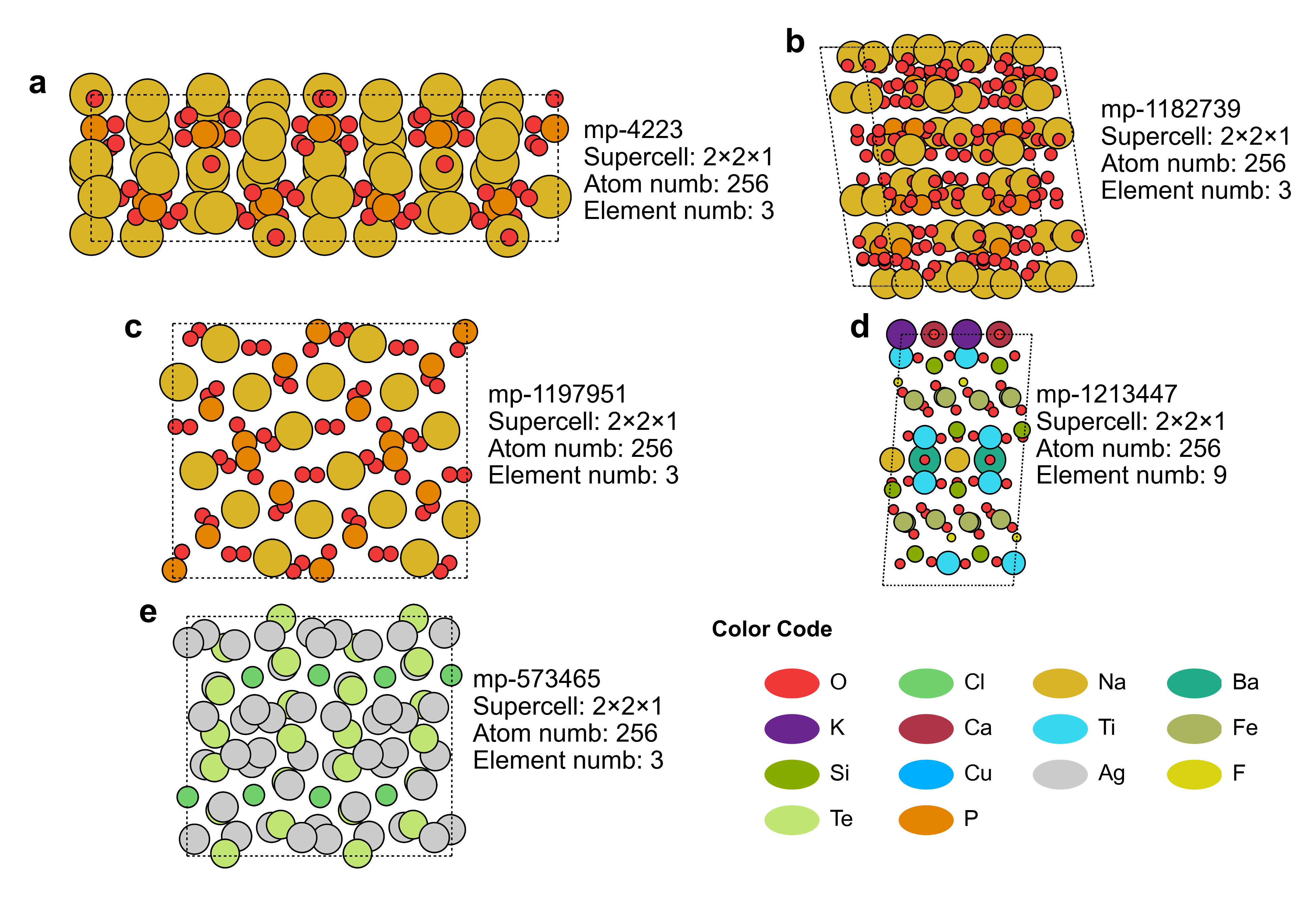
Benchmark structures with five configurations: (a)–(e) feature different elemental compositions while maintaining an identical atom count (N = 256). Each configuration was tested separately, and the average metrics were reported.